This Long-Form Post is my personal reference guide on Investing, consolidating materials and experiences I’ve come across over the years into my own Investing Philosophy and Process.


This post is a work-in-progress.


My investing philosophy in 1 paragraph:

Value and momentum are main drivers of returns while diversification reduces risks and thinking about the long term helps reduce negative behavioural biases.

Investment Philosophy & Process
Valuation

Valuation is a good indicator of long term returns. Valuation plays take time to work out and typically we are looking at 3-5 years.


Valuation is a timeless concept and would adapt to suit almost any regimes. There have been numerous empirical investigations and conclusions to show the merits of basic valuation measures on both Equities and Bonds. Basic valuation measures include Cyclically Adjusted Price to Earnings, Price to Earnings and Dividend Yields for Equities and Current Yield relative to consensus GDP for Bonds.


CAPE is a reliable long term valuation indicator for both developed and emerging markets and can be used to predict real returns on local equity markets over the next 5 years. The relationship between the CAPE and future real stock market returns seems to depend very much on the prevailing macroeconomic regime. Particularly an environment of rising interest rates seems to lead to generally lower real returns for stock markets given a specific level of the CAPE. (Wellershoff & Partners)

Momentum

Absolute and relative momentum works better over a shorter time horizon compared to value investing.


Trends often experience periods of increased volatility as they become more profitable. We believe it is necessary to endure these periods of volatility in exchange for greater returns in the long run.

Factors and Risk premiums

Factors are the building blocks of the portfolio.


Equity premium deliver a persistent premium through time.

Diversification

Diversification helps to lower overall risk of a portfolio when different asset classes or strategies with low or negative correlation are put together.


A related concept which should be briefly discussed here is the difference between investing in the “market” and investing in individual securities or companies. When we invest in “markets” instead of individual companies, the idiosyncratic risk is broadly diversified. There is much lesser chance of the “market” going into prolonged depression and “bankruptcy”. To put it in another manner, a cheap company may be “cheap” for a long time and eventually goes out of business. A cheap market has much lesser chance of being “cheap” for a prolonged period.

Disciplined Investing

Important to have a clear set of rules to guide your decision making.

Market psychology

Financial markets are driven by investor psychology and the most important thing psychology tells us is that people learn almost nothing from history.

The market is made up of people, and to beat it you have to know them as well as you do the thing you are considering investing in.

While investing draws on knowledge of accounting, economics and finance, it also requires insight into psychology. Why? Because investors’ objectivity and rationality rarely prevail as much as investment theory assumes, and emotion and “human nature” often take over instead.

Price

“Price is a liar”.


The human mind wants to come up with a unifying theory to explain complexity. Price is all the information that exists in the market.


He thinks that price means nothing other than the equilibrium of liquidity (buyers and sellers, supply and demand). It doesn’t mean good or bad, it’s just where people agree.


Hence price as it moves gives you tremendous opportunities. Current liquidity (demand and supply) does not reflect the future and the further up the future or the more extraordinary the future the less current price matters.


Price is full of risks; one direction or the other.

Risk

Risk is the chance of permanent loss. Volatility is the typical measure for risk but must be broken into upside and downside volatility. Upside volatility should not be penalized.


Capital Preservation is important.

Predictions and Forecasting

Predictions and forecasting is very hard. It is easier to accept that prediction is impossible and build robust portfolios with the understanding that black swan events happen quite commonly.


As Oaktree Capital Management’s Howard Marks says: “You cannot predict but you can prepare”


We have two classes of forecasters: Those who don’t know and those who don’t know they don’t know.

Simplicity over Complexity

Simple approaches tend to be more robust compared to complex approaches.

Liquidity

Liquidity is the ability to execute an order of a given size, at a chosen point in time and with relative ease (or minimal cost).

Second level thinking

There is nothing reliable to be learned about making money. If there were, study would be intense and everyone with a positive IQ would be rich. – John Kenneth Galbraith


Anyone who thinks it’s easy to make money from markets must be a first level thinker.
First-level thinking says:”It’s a good company; let’s buy the stock.” Second level thinker says: “It’s a good company but everyone thinks it’s a great company, and it’s not. So the stock is over-rated and over-priced. Let’s sell”


First level thinking is simplistic and superficial. First level thinkers see what’s on the surface, react to it simplistically and buy or sell on the basis of their reactions. They don’t understand their setting as a marketplace where asset prices reflect and depend on the expectations of the participants. They ignore the part that others play in how prices change. And they fail to understand the implications of all this for the route to success.


The herd is wrong about risk as often as it is about return. When everyone believes that something is risky; their unwillingness to buy usually reduces its price to the point where it’s not risky at all. This paradox exists because most investors think quality, as opposed to price, is the determinant of whether something’s risky. But high quality assets can be risky, and low quality assets can be safe. It’s just a matter of the price paid for them.


The riskiest thing in the world is the widespread belief that there’s no risk.


The problem that befalls most people (the first level thinkers) is that they fail to distinguish between fundamental risk and investment risk. What has to be remembered is the defining role of price. Regardless of whether the fundamental outlook is positive or negative, the level of investment risk is determined largely by the relationship between the price of an asset and its intrinsic value.

Market Analysis
Sovereign Yields

sovereign-yields-080116

Sovereign Term Spreads

sovereign-term-spread-080116

Equities Valuation - Market Cap to GDP

mkt-cap-to-gdp-080116

Equities Valuation - Cyclically Adjusted Price to Earnings

cape-120116

Equities Valuation - Dividend Yield

dividend yield monitor 090316

Risk Indicators

vix and sp500 sectors goldman

Trading System Design
Simplicity Over Complexity

The less rules your system contains the more robust your strategy will be in real trading.

Risk Management - Stop-Loss

To determine stop-loss level, use Maximum Adverse Excursion. MAE is defined as the most intraday price movement against your position. Plot cluster Y-axis Profits, X-axis Drawdown. Try to use the optimal stop loss distance. The same method can be used for trailing stop etc.


Trailing Stop is a dynamic order that moves up with new highs or down with new lows in the market so as to preserve some predetermined proportion of open trade profit.


Trailing Dollar Profit Stop is an order to exit a position and set at a fixed dollar value above the most current low price (short) or below the most current high price (long).


Trailing volatility profit stop is an order to exit a position and set at a point value based upon some measure of market volatility above the most current low price (short) or below the most current high price (long).

Risk Management - Profit-Target

Profit target is an unconditional exit of a trade with a locked in profit at some predetermined price or profit level.


In general active counter trend trading strategies that trade from overbought and oversold conditions benefit the most from profit target orders. Slower trend following trading strategies benefit the least from profit targets.


Dollar profit target is an unconditional exit of  a trade at a profit and at a price level equal to a dollar amount above (long) or below (short) the entry price.


Volatility profit target is an unconditional exit of a trade at a profit and at a price level equal to a value based upon market volatility above (long) or below (short) the entry price.

Risk Management - Compounding

In system development, fixed size trades should be used. Compounding introduces a distortion that encourages selection of system that will not perform well out of sample.

Position Sizing
Fixed Size

Fix the number of lots.


Maximum Drawdown

Have enough equity to withstand the worst case maximum drawdown.

Take 150% of the worst case drawdown plus the margin for the first lot. Each subsequent lot is added when the equity increase by 150% of the worst case drawdown.


Fixed % Size

Risk the same percentage on each trade.


Fixed Ratio

Key parameter is Delta, the dollar amount of profit per traded unit to increase the number of units by one.

Base to calculate the number of traded lots is
N = 0.5 * [((2 * No – 1)2 + 8 * P/delta)0.5 + 1]
where N is traded position size, No is starting position size, P is total closed profit, Delta is as above.


Optimal F

Fixed fractional trading, introduced by Ralph Vince, based on formula derived from Kelly method.


Kelly Formula

Kelly% = (win% – loss%)/(average profit/average loss)

Due to limited sample size and large variance, the numbers used in this formula will introduce a significant degree of variance in the results of the Kelly formula. It is this very fuzziness that introduces a level of inaccuracy in the use of formulae such as Kelly or Optimal F.


Safe f

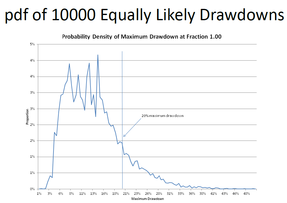
We want max safe position size with regards to risk tolerance. Too high a position size and drawdown is likely to exceed tolerance, too low a position size and we voluntarily sacrifice profits.
safe-f-1

safe-f-2

safe-f-3

The Only Knob to turn to achieve the optimal risk level is Position Size. Lowering position size lowers drawdown. Fractional position sizing is near-optimal and easily implemented.


For the test so far, all trades were taken with all funds. Position size = 1.00 which means full fraction. Position size is not stationary, but for now assume one position size works equally well over the entire time period.


What fraction is safe?

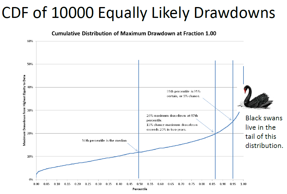
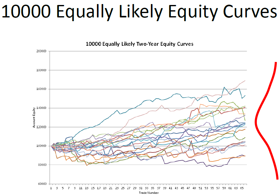
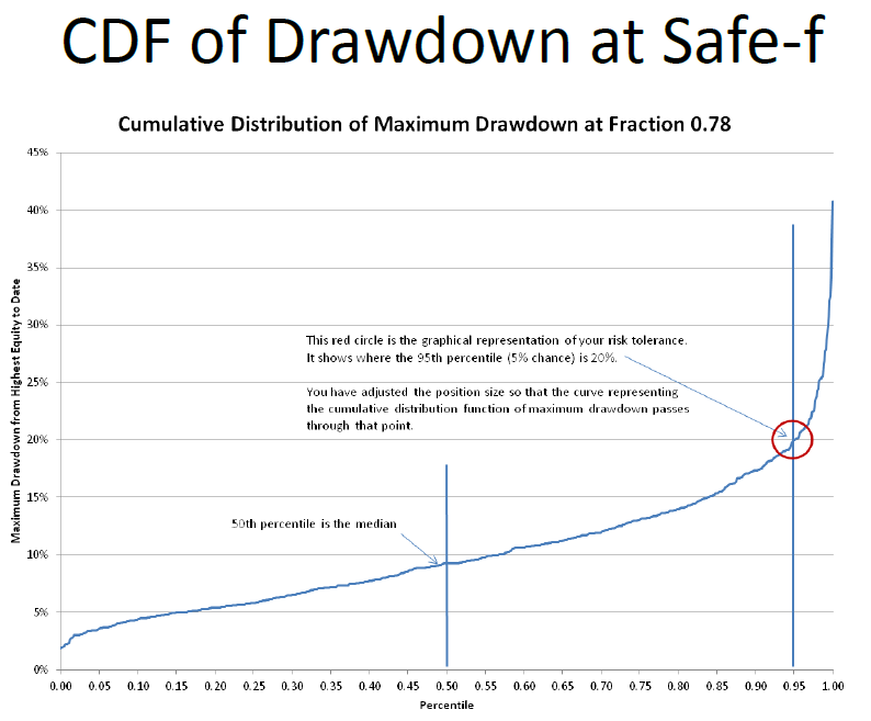
Using Monte Carlo of 2 years, we do not know which patterns will occur in which order over the next two years.  The set of 423 trades from the development tests we are analyzing is our “best estimate.” It covers 13 years. At random, pick enough trades from the 423 to cover 2 years – 65 trades. The position size that lowers drawdown to the point you feel the system is safe to trade is safe-f.

Profit is a function of position size. You want the highest position size fraction you can tolerate. We want to limit drawdown in the balance of the entire trading account.


If safe-f is less than 1.00, some funds will be left in cash as ballast. They cannot be used for any other purpose. The drawdown of the combined traded plus ballast is 20%.

  • Drawdown of ballast is 0%.
  • Drawdown of traded funds is approximately 20% / safe-f.
  • Adjust Position Size
  • Rerun the Monte Carlo simulation using different values for the fraction.
  • Search for the highest fraction where maximum drawdown is 20% at the 95th percentile.
  • For this system, that fraction, safe-f, is 0.78.
 

safe-f-4

Back-testing - Verification Of Trading Ideas

We want to see whether it works on past historical data. We also want to develop an opinion of the likelihood that the trading strategy will produce real time profits in a proportion similar to that of its historical profile.


We are also interested to see what the profits and risks of the trading strategy is over both ever changing market conditions and different markets. If we find that the trading strategy produces profit over a range of conditions (necessary) and a variety of markets (desirable but not necessary), we have further validation of the trading concept.


In contrast let us consider what is likely to follow if we begin our trading adventure with a bunch of vague, inconsistent, and unverified ideas. First, such a configuration cannot be tested. We have only our faith in the merits of the trading ideas. We have no solid knowledge of their past effectiveness or of their risk and return.


Even the discretionary trader trades with a plan and systematically determines entries, exits, trade size, and so on.


Trading without a well defined plan has the same likely outcome as doing anything without a plan. Failure.

Back-testing - Platforms

Common platforms include:

Python Language

Tradestation

MetaStock

Amibroker

MatLab

R

Multicharts

Wealth-lab

Mechanicasoftware

Rightedge

Back-testing - Data

Common data sources include:
CSI Data, Pinnacle Data, Interactive Data, https://quantgo.com

Back-testing - Test Time Horizon

Test data should cover a full market cycle and different price regimes. More recent data is more relevant and valid. Price series must be long enough to entail different market situations and to produce a significant number of trades.
Standard Error = S.D / Sqr Root of the sample size


Degree of freedom:
Number of variables and conditions and the data used should not be more than 10% of the whole data sample considered.


Degree of freedom = whole data sample – rules and conditions – data consumed by rules and conditions


Start Up Cost:
Direct impact on sample size independent of issues of degrees of freedom. A trading signal cannot occur until there are enough data points to have for e.g. moving averages.


Statistical Soundness:
Large enough to generate statistically sound results. Include a broad sample of data conditions. Large number of trades so as to be able to draw meaningful conclusions. Large enough to allow enough degree of freedom for the number and length of the variables employed by the trading strategies. Relevance to trading system and market.

Back-testing - Market Selection

Best to select a basket of highly diversified markets.

  • Statistical correlation Rule of thumb: +0.5 to -0.5
  • Fundamental diversity


Chesapeake: All the markets they trade are exchanged traded, centrally cleared and marked to market daily. They invest in over 100 futures markets worldwide. These markets include stock indices, single stocks, interest rates, currencies, grains, meats, metals, energies and softs. These markets are geographically dispersed.

Back-testing - De-trending

In a bullish bias market regime, a long bias system does better and performance is over rated. A poor performance for a short bias system is under rated.


We need to detrend the price series for better analysis. It is also important to realise how often the system is in the market. If the trade holding period is very short and is in the market less than 10% of the time in total, the impact of market bias is less significant.


Detrended price series should only be used for calculating returns. Signal generation is still done on actual price series.


Minus the mean returns from each daily price return to detrend. Use log(current day price/ prior day price) to get daily prices.

Back-testing - Stability and Consistency

Trading strategy performance is more stable when:

  • Trades/Profits are relatively evenly distributed throughout the test window.
  • The standard deviation of the size and the length of wins and losses is smaller.
  • The trading performance is consistent from parameter set to parameter set.
  • There is a balance between long and short profits.
  • There are relatively stable winning and losing runs.
  • There are large and statistically valid number of trades.
  • There is positive performance trajectory.

1. Calculate the average, standard deviation, maximum, minimum for each of important indicators. The smaller the span between the max and min and the smaller the standard deviation, the smaller therefore is the variance and hence the more consistent the performance of the trading strategy.
2. Remove the maximum value from each category and then recalculate the average without it. If this adjusted average is considerably smaller (1 to 2 SD) than unadjusted average, this suggests excessive influence by the maximum.
3. Determine how well spread out each of these performance measures are throughout the historical time period under review.

Robustness test:

  1. A broad range of contiguous parameter sets
  2. Wide ranging basket of diverse markets
  3. Wide range of market types and conditions
  4. Long and short trades
Back-testing - Key Objective Function
Pessimistic Return On Margin (PROM)
  • Annualised yield on margin that is adjusted in a way that pessimistically assumes that a trading strategy will win less and lose more in real trading than it did in its historical simulation.
  • #WT = Number of wins
  • AW = Average win
  • #LT = Number of losses
  • AL = Average loss
  • PROM = {[AW * (#WT – Sq(#WT))] – [AL * (#LT – Sq(#LT))]} / Margin


PROM Variants
  • PROM minus biggest win removes the largest single profitable trade from the gross profit and is then calculated according to the same formula as PROM.
  • PROM minus the biggest winning run removes the gross profit of the largest run of winning trades from the gross profit and is then calculated with the same formula as PROM.


Risk Adjusted Returns
  • Annualised RAR = Annualised Profit / (Margin + Max DD * 2)


Reward to Risk Ratio
  • RRR = Net Profit / Max DD
  • A bigger RRR implies that reward per trading dollar is increasing relative to the risk.


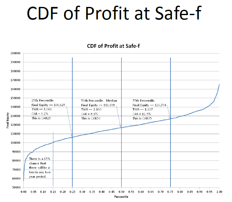
CAR25
  • Distribution of Profit
  • What is the profit, when each trade is taken using 78% of available funds?

safe-f-5


Others
  • Net Profit
  • Profit factor
  • Average trade profits in %
  • Percentage of profitable trades
  • Average DD
  • Max DD
  • We can also determine the max DD to be how many St Dev of the average DD. If its 1 or 2 SD from mean we can reasonably expect such DD to occur. If it is beyond 2 SD we may need to rethink the logic of the system
  • Average holding period.
  • Number of trades
Back-testing - Walk Forward Analysis

Walk forward analysis is a kind of multiple and successive out of sample test over the same data series. Equity line resulting from walk forward run is where we are closest to reality. It is out of sample. WFA judges the performance of a trading system exclusively on the basis of post optimization or out of sample trading. Trading strategy is first optimized on a historical sample then traded on a new and unseen historical sample. Known as out of sample testing.

Anchored WFA
Starting period always the same and the optimisation period gets longer and longer as the time goes by


Rolling WFA
More suitable for intraday strategies.


Length of time a model can be traded in real time before requiring optimisation:
Those built on bigger optimisation windows are said to have longer life in real trading. A shorter window requires more frequent optimisations, is more responsive, more profitable to current price action and less capable of adapting effectively to dramatic changes in trend and volatility. A longer window requires less frequent reoptimization, less responsive, less profitable to current price action and is more able to adapt effectively to large shifts in trend and volatility. A good rule of thumb for the determination of the size of the trading window is to set it at between 1/8 and 1/3 of the test window size. A strategy optimized properly on 2 years of price history will likely remain usable for between 3 to 6 months of real life trading. If the walk forward window is 3 windows then the model must be reoptimized at the end of every 3 months of trading and so on for different window sizes. Main reason a trading system must be reoptimised is that markets change with some frequency. The do not change with great regularity.


To gauge the forecasting power of the system and its consistency, calculate the ratio between the annualised net profit relating to the walk forward tests and the annualised net profit during the optimisation periods. This is the walk forward efficiency ratio. A unique measurement of the quality of the actual optimization process. Compares the annualised rate of postoptimization profit with that of in-sample optimization profit.  Above 100% is efficient. If 50% then expect a system to perform half as well. 50% normally used as minimum efficiency. Do as many number of walk forward analysis tests as possible, or at least 10 tests with a test window of about 20% of the whole optimisation price series.

Optimisation

Optimisation is good if done in a savvy way. Curve fitting is optimisation gone wrong. Optimisation is the process whereby a trading strategy is tested and refined so as to produce the best possible real time trading profits. Optimisation comes after testing. We will determine that a strategy is sound before we perform optimisation. The lesser parameters the better. The more parameters the higher the risk of curve fitting.

Optimisation Framework
  • The strategy parameters that are to be used in the optimization must be selected and the scan ranges to be used must be determined.
  • The greater the number of parameters to by optimized, the more likely it is that the results will be overfitted or optimized incorrectly.
  • A parameter is important if such a scan shows dramatic performance changes.
  • Keep the step sizes of each parameter to be scanned somewhat proportional to one another. Put the step scan range in an almost parallel relationship so that the scan from 1 to 20 will be performed with a step of 2 and the scan from 20 to 200 will be performed with a step of 20.
  • Over scanning occurs when a parameter scan uses a step size that is too small or steps over a range that is too large.
  • Appropriate data sample must be selected.
  • Objective function that identify the best parameters for the trading strategy must be selected.
  • Guidelines for the evaluation of the optimization process must be determined.
  • Optimization is robust when optimization profile has some degree of statistical significance. i.e. enough profitable parameters sets in the optimization profile. Results are statistically significant and not simply the product of chance.
  • The more evenly distributed and the smaller the variation of performance from parameter set to parameter set, the more robust the trading strategy is.
  • Robustness of an optimization profile lies in the shape and contour of the optimization. A profit spike surrounded by poor performance is unlikely to be a robust strategy capable of producing real time profit. The more robust trading strategy will have an optimization profile with a large average profit, small maximum-minimum range and small standard deviation. Other indicators are count, average, total and standard deviation of net profit and loss of all trades and of all profitable trades.
Optimisation Search Methods
Grid Search
  • Simplest form, most common.
  • Brute force, simply calculates and then ranks every historical simulation.


Prioritised Step Search
  • Scans one parameter at a time while holding a selected value constant for each of the other parameter ranges.
  • Then choose best value for first parameter and vary the other.
  • Can repeat the whole steps multiple iterations.


Hill climbing Search Algorithms
  • Enlightened or informed selectivity. A hill climbing search follows a path of increasing performance in the optimization space.


Multipoint Hill Climbing Search
  • Doing multiple hill climbing searches, each starting at a different point in the optimization space.


Simulated Annealing
  • Advanced directed search method modeled after the cooling of molten metals which as their heat slowly escapes, tend to crystallise into patterns that minimize their own internal energy states.


Genetic Algorithms
  • Class of advanced search methods that emulate the biological process of evolution.


Particle Swarm Optimization
  • Based on the observed behavior of flocks of birds and schools of fish.
  • Family of stochastic search methods.
Overfitting

Overfit trading strategy will produce very impressive results during simulation and often devastating poor performance during real time trading. Walk Forward Analysis evaluates performance of the trading strategy on price data that was not part of the optimization process. There are still those who derisively and with great ignorance dismiss all optimization as over fitting. An overfit strategy is one that is excessively fit or fit to an unwanted degree and not suitable or appropriate for the purpose of producing real time trading profits. It produces good trading performance on in sample price history but produces poor trading performance on out of sample price history. It is essential to rigourously follow correct testing and optimization procedures. Optimization refers to a properly executed optimization that identifies parameters that are the most capable of producing real time trading profits.


Causes of overfitting

  • Insufficient degrees of freedom
  • Inadequate data and trade sample
  • Incorrect optimization methods
  • Big win in a small trade sample
  • Absence of Walk Forward Analysis


Chesapeake: We believe research can yield systems that are clever, complex and perform magnificently on historical data, but in real‐time they do not have those same returns. We believe each additional parameter merely extracts, or cherry‐picks, attractive subsets of trades in a pattern unlikely to be reproduced in real‐time.

Proper Capitalization

An account must be funded with sufficient capital to absorb the maximum risk or drawdown that the trading system must endure. Required capital is the amount of trading capital necessary to accommodate max DD, margin requirements, and a safety factor so as to successfully trade with a strategy.

  • Calculated as Max DD * safety factor (1.5) * 2 + Margin.
  • Able to weather back to back Max DD
  • Or using a strategy stop loss, Required Capital = (Max DD*Safety Factor)/Capital Stop e.g. 40%)
Portfolio Construction - Weighting
  • Equal Weighting
  • Weighted by largest drawdown
  • Weighted by expected drawdown
  • Compose portfolio by normalising risk by the largest losing trade or drawdown. A risk parity concept.
Portfolio Construction - Correlation
  • Check negative or low correlation between equity lines.
  • Measure the inter correlation of daily equity changes among the different market systems.
  • Combining uncorrelated systems increases the ratio of expected returns to expected risk.
  • Prefers different strategy types. (e.g. trend, mean reversion, momentum)
  • Calculate average correlation of the matrix. Rule of thumb is < 0.2.
  • The proper way to do it is to run the correlation on the natural log returns, not on the percentage returns and definitely not on the price. R(i) = Ln(P(i)/P(i-1))
Portfolio Construction - Coincident negative return (CNR) matrix

Coincident negative return (CNR) matrix

  • Shows the percentage of time the investment in that row was down, given the column investment was down.
  • Non symmetrical.
  • Define the maximum loss threshold (T). Default is zero, any loss would represent a losing month. Can use a higher threshold such as -0.5%.
  • If Fund C was down in 20% of all months and in 60% of those same months, Fund E was also down, then the value would be 60%.


Normalising CNR

  • The significance of what percentage of the time a manager loses when another manager loses depends on whether this percentage is more or less than the manager’s average percentage of losses.
  • Normalise: Each percentage is divided by a manager’s average percentage of losses worse than the threshold (T).
  • If Manager A is down in 30% of all months but in only 20% of the months when Manager B is down, the normalise CNR is 66.7% (20%/30%).
Portfolio Implementation

Performance of a trading strategy in real time must be compared to that of competing strategies and investments.


Real time performance can decline for 3 reasons

  1. It is a poor trading strategy
  2. Market opportunity has contracted
  3. Unseen market conditions have emerged
Emotions

Who complains about a windfall profits? No one. However do not let greed and ego get the upper hand in such a fortunate situation. Such a large profit is typically a windfall. Who complains when real time trading begins with a losing streak? Almost everyone. With such a start a trader may panic and often without justification. The onset of real time trading can begin with a winning or losing run. Consider a third case, a trading strategy produces a run of uneventful wins and losses producing a small net gain or loss after the first month of trading. This type of activity can prove almost as trying. Traders are not known for their patience. No matter which way it starts, if its performance is in alignment with its evaluation profile, it is all good.

Life Cycle Of Trading Strategies

First school of thought maintains that the only good trading strategy is a trading strategy that need not and does not vary over time. Inherent in this belief is that the best trading strategy will work without optimization and on all markets with the same rules and parameters. The alternative view is that to achieve optimal trading performance over long periods of time with a trading strategy, it will need to be updated occasionally. Trader should be constantly looking to change, adapt, and develop his strategies. Models and strategies will benefit from modification from time to time.